platform for control and data acquisistion application development

Introduction

In this article, we will show how to use DSP management tools. We will show FFT example where the analog signal is generated on analog output and acquired with DSP management functions. MicroDAQ toolbox provides macros for managing DSP execution, a user can load DSP binary from Scilab script, register signal, read data from running DSP application and terminate its execution. This way application can be divided into a real-time part, which is executed on MicroDAQ DSP and script which allows using all Scilab functions for calculations. The FFT example uses Xcos generated DSP application and Scilab FFT function which calculates FFT from real-time data.

Xcos model

Our application will calculate FFT from real-time DSP data., we will start from creating example model which generates analog signal with two sine waveforms with different amplitude and frequency.

The diagram contains two sine waveform generators which output is added and passed to DAC block. Then we use ADC block to read analog samples from DAC (analog input and output should be wired). Data from ADC block is passed to SIGNAL block which sends data to host and this data can be read from Scilab script. Our model will run with 5kHz. After model creation, we generate DSP application by selecting Tools->MicroDAQ build model. The resulting application will be used in Scilab script for FFT calculation.

Running DSP application from Scilab script

MicroDAQ toolbox for Scilab provides macros which manage DSP execution. These macros can be used with a standard script to run DSP application in parallel with a Scilab script.

DSP managment scilab macros:

• mdaqDSPStart(path, rate) - starts DSP binary from path with rate
• mdaqDSPStop() - terminates DSP execution
• mdaqDSPSignal(id, size) - registers Xcos signal
• mdaqDSPSignalRead(count) - reads Xcos signal
• mdaqDSPBuild(path) - builds DSP binary from Xcos model
  

The example Scilab script which uses Xcos generated DSP application:

 1
 2
 3
 4
 5
 6
 7
 8
 9
10
11
12
13
14
15
16
17
18
19
20
21
22
23
24
25
26
27
28
29
30
31
32
33
34
35
36
37
38
39
40
41
42
43
44
45
46
47
48
49
50
51
52
53
54
55
56
57
58

duration = 20;
rate = 5000;

// Build DSP binary from Xcos model
mdaqDSPBuild(mdaqToolboxPath() + filesep() + "examples" + filesep() +"fft_demo.zcos");

// Start DSP application
result = mdaqDSPStart('fft_demo_scig\fft_demo.out', 1.0/rate);
if result < 0 then
    abort;
end

// Register signal ID and signal size
result = mdaqDSPSignal(1, 1);
if result < 0 then
    disp("ERROR: unable to register signal");
    abort;
end

first_time = 1;
a = [];

// Process data from DSP
sample_count = FREQ/10;
fig = figure("Figure_name","MicroDAQ FFT demo");

for i=1:(duration*10)
    [result, s] = mdaqDSPSignalRead(sample_count);
    if result < 0 then
        disp("ERROR: unable to read signal data!");
        abort;
    end

    N=size(s,'*');  //number of samples
    s = s - mean(s);//cut DC
    y=fft(s');

    f= FREQ*(0:(N/10))/N; //associated frequency vector
    n=size(f,'*');

    if is_handle_valid(fig) then
        if first_time == 1 then
            clf();
            plot(f,abs(y(1:n)));
            title("FFT", "fontsize", 3);
            xlabel("frequency [Hz]","fontsize", 3);
            first_time = 0;
            a = gca();
        else
            a.children.children.data(:,2) = abs(y(1:n))';
        end
    else
        break;
    end
end

// Stop DSP execution
mdaqDSPStop();

Our script loads DSP application with mdaqDSPStart() macro which as an argument takes Xcos generated DSP binary path and model rate. When the user provides -1 as a rate argument model rate the default model rate defined in Xcos model will be used. After this call DSP binary will be loaded and started on MicroDAQ DSP. In order to have access to signal data we have to register signal with mdaqDSPSignal() macro which takes two arguments, first one is signal ID defined in Xcos SIGNAL block and the second one is signal vector size which has to match with Xcos signal size. The script will read 500 samples from DSP and makes FFT calculation on this data. The mdaqDSPSignalRead() macro reads signal data from DSP, it needs one parameter which is data count which defines how many vectors will be read from DSP. The mdaqDSPSignalRead() will block Scilab until requested data is received. Reading DSP samples and FFT calculation is done in a loop. Our DSP application runs with 5kHz frequency so every 1/10sec we will new 500 samples from DSP and plot will be updated with new FFT result. After for loop completion, we need to terminate DSP execution with mdaqDSPStop() macro.

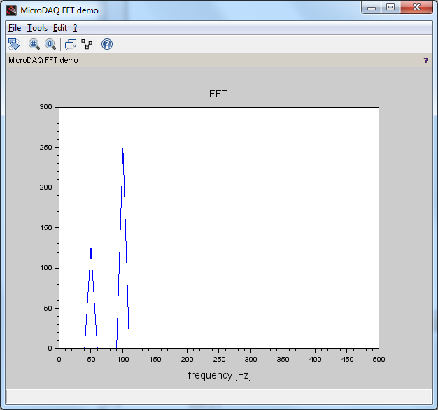
As expected on FFT plot we can see peaks at 50Hz and 100Hz with different amplitude. 

Learn more:

Online documentation

Real-time processing with Scilab script - Video